Generate random graphs according to the \(G(n,p)\) Erdős-Rényi model

Every possible edge is created independently with the same probability p. This model is also referred to as a Bernoulli random graph since the connectivity status of vertex pairs follows a Bernoulli distribution.

Usage

sample_gnp(n, p, directed = FALSE, loops = FALSE)

gnp(...)

Arguments

n

The number of vertices in the graph.

p

The probability for drawing an edge between two arbitrary vertices (\(G(n,p)\) graph).

directed

Logical, whether the graph will be directed, defaults to FALSE.

loops

Logical, whether to add loop edges, defaults to FALSE.

...

Passed to sample_gnp().

Value

A graph object.

Details

The graph has n vertices and each pair of vertices is connected with the same probability p. The loops parameter controls whether self-connections are also considered. This model effectively constrains the average number of edges, \(p m_\text{max}\), where \(m_\text{max}\) is the largest possible number of edges, which depends on whether the graph is directed or undirected and whether self-loops are allowed.

References

Erdős, P. and Rényi, A., On random graphs, Publicationes Mathematicae 6, 290–297 (1959).

See also

Random graph models (games) bipartite_gnm(), erdos.renyi.game(), sample_(), sample_bipartite(), sample_chung_lu(), sample_correlated_gnp(), sample_correlated_gnp_pair(), sample_degseq(), sample_dot_product(), sample_fitness(), sample_fitness_pl(), sample_forestfire(), sample_gnm(), sample_grg(), sample_growing(), sample_hierarchical_sbm(), sample_islands(), sample_k_regular(), sample_last_cit(), sample_pa(), sample_pa_age(), sample_pref(), sample_sbm(), sample_smallworld(), sample_traits_callaway(), sample_tree()

Author

Gabor Csardi csardi.gabor@gmail.com

Examples

# Random graph with expected mean degree of 2
g <- sample_gnp(1000, 2 / 1000)
mean(degree(g))
#> [1] 2.028
degree_distribution(g)
#> [1] 0.136 0.257 0.274 0.185 0.096 0.034 0.013 0.004 0.001

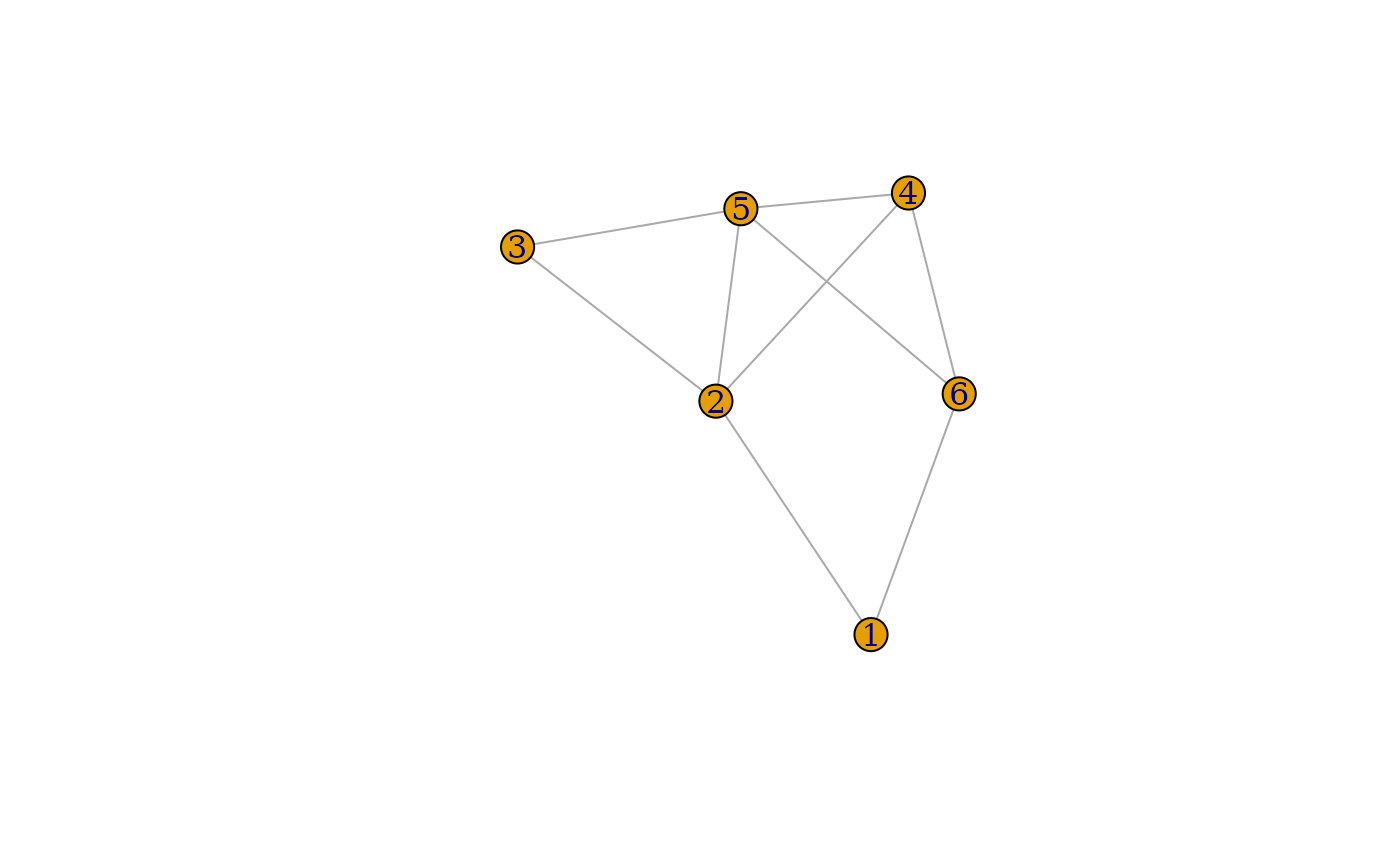
# Pick a simple graph on 6 vertices uniformly at random
plot(sample_gnp(6, 0.5))