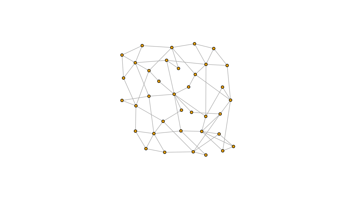
Place vertices of a graph on the plane, according to the simulated annealing algorithm by Davidson and Harel.
Usage
layout_with_dh(
  graph,
  coords = NULL,
  maxiter = 10,
  fineiter = max(10, log2(vcount(graph))),
  cool.fact = 0.75,
  weight.node.dist = 1,
  weight.border = 0,
  weight.edge.lengths = edge_density(graph)/10,
  weight.edge.crossings = 1 - sqrt(edge_density(graph)),
  weight.node.edge.dist = 0.2 * (1 - edge_density(graph))
)

with_dh(...)
Arguments
- graph
The graph to lay out. Edge directions are ignored.
- coords
Optional starting positions for the vertices. If this argument is not
NULLthen it should be an appropriate matrix of starting coordinates.- maxiter
Number of iterations to perform in the first phase.
- fineiter
Number of iterations in the fine tuning phase.
- cool.fact
Cooling factor.
- weight.node.dist
Weight for the node-node distances component of the energy function.
- weight.border
Weight for the distance from the border component of the energy function. It can be set to zero, if vertices are allowed to sit on the border.
- weight.edge.lengths
Weight for the edge length component of the energy function.
- weight.edge.crossings
Weight for the edge crossing component of the energy function.
- weight.node.edge.dist
Weight for the node-edge distance component of the energy function.
- ...
Passed to
layout_with_dh().
Value
A matrix with two columns, containing the x and y coordinates of the vertices:
- x
The x-coordinate of the vertex.
- y
The y-coordinate of the vertex.
Details
This function implements the algorithm by Davidson and Harel, see Ron Davidson, David Harel: Drawing Graphs Nicely Using Simulated Annealing. ACM Transactions on Graphics 15(4), pp. 301-331, 1996.
The algorithm uses simulated annealing and a sophisticated energy function, which is unfortunately hard to parameterize for different graphs. The original publication did not disclose any parameter values, and the ones below were determined by experimentation.
The algorithm consists of two phases, an annealing phase, and a fine-tuning phase. There is no simulated annealing in the second phase.
Our implementation tries to follow the original publication, as much as possible. The only major difference is that coordinates are explicitly kept within the bounds of the rectangle of the layout.
References
Ron Davidson, David Harel: Drawing Graphs Nicely Using Simulated Annealing. ACM Transactions on Graphics 15(4), pp. 301-331, 1996.
See also
layout_with_fr(),
layout_with_kk() for other layout algorithms.
Other graph layouts:
add_layout_(),
component_wise(),
layout_(),
layout_as_bipartite(),
layout_as_star(),
layout_as_tree(),
layout_in_circle(),
layout_nicely(),
layout_on_grid(),
layout_on_sphere(),
layout_randomly(),
layout_with_fr(),
layout_with_gem(),
layout_with_graphopt(),
layout_with_kk(),
layout_with_lgl(),
layout_with_mds(),
layout_with_sugiyama(),
merge_coords(),
norm_coords(),
normalize()
Author
Gabor Csardi csardi.gabor@gmail.com
Examples
set.seed(42)
## Figures from the paper
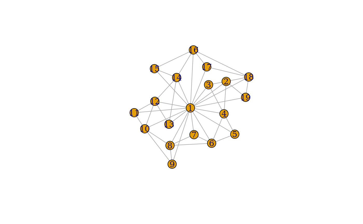
g_1b <- make_star(19, mode = "undirected") + path(c(2:19, 2)) +
path(c(seq(2, 18, by = 2), 2))
plot(g_1b, layout = layout_with_dh)
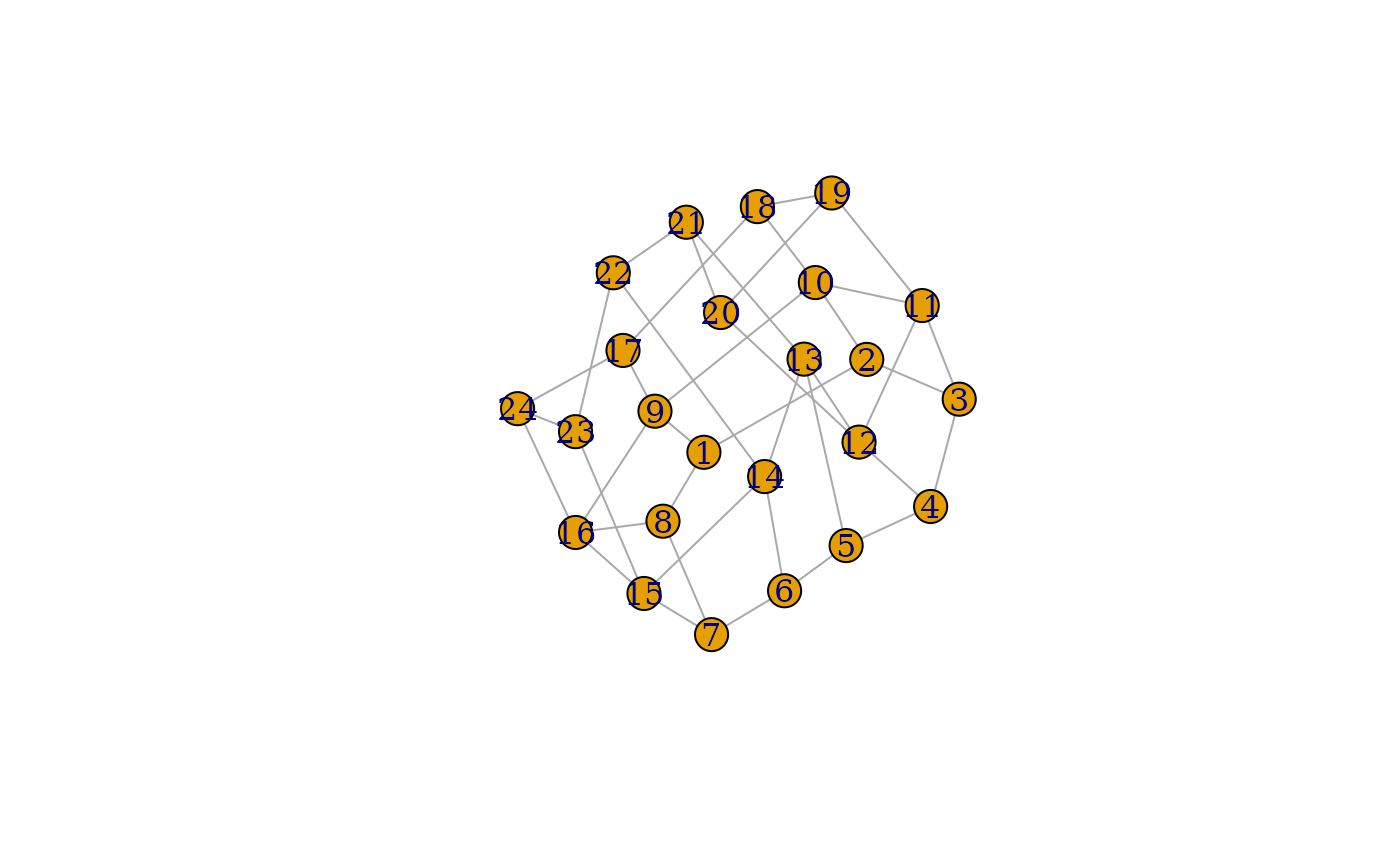
 g_2 <- make_lattice(c(8, 3)) + edges(1, 8, 9, 16, 17, 24)
plot(g_2, layout = layout_with_dh)
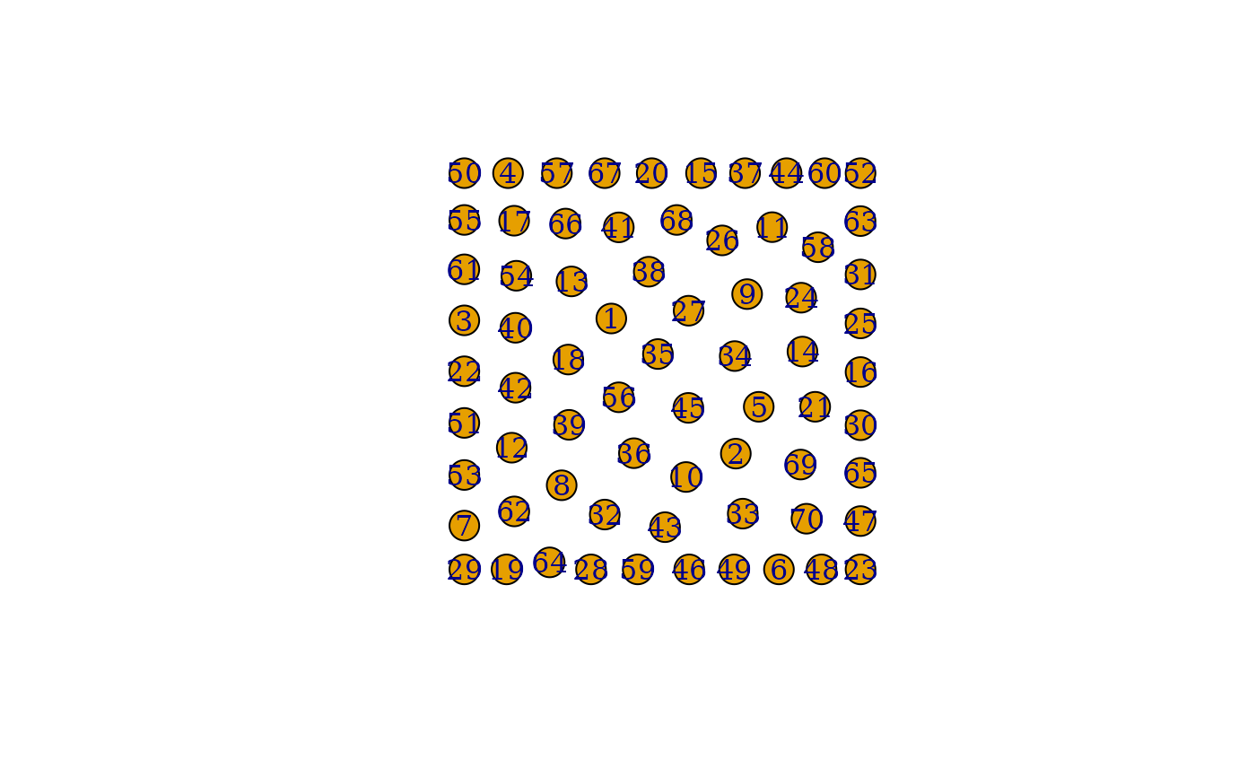
 g_3 <- make_empty_graph(n = 70)
plot(g_3, layout = layout_with_dh)
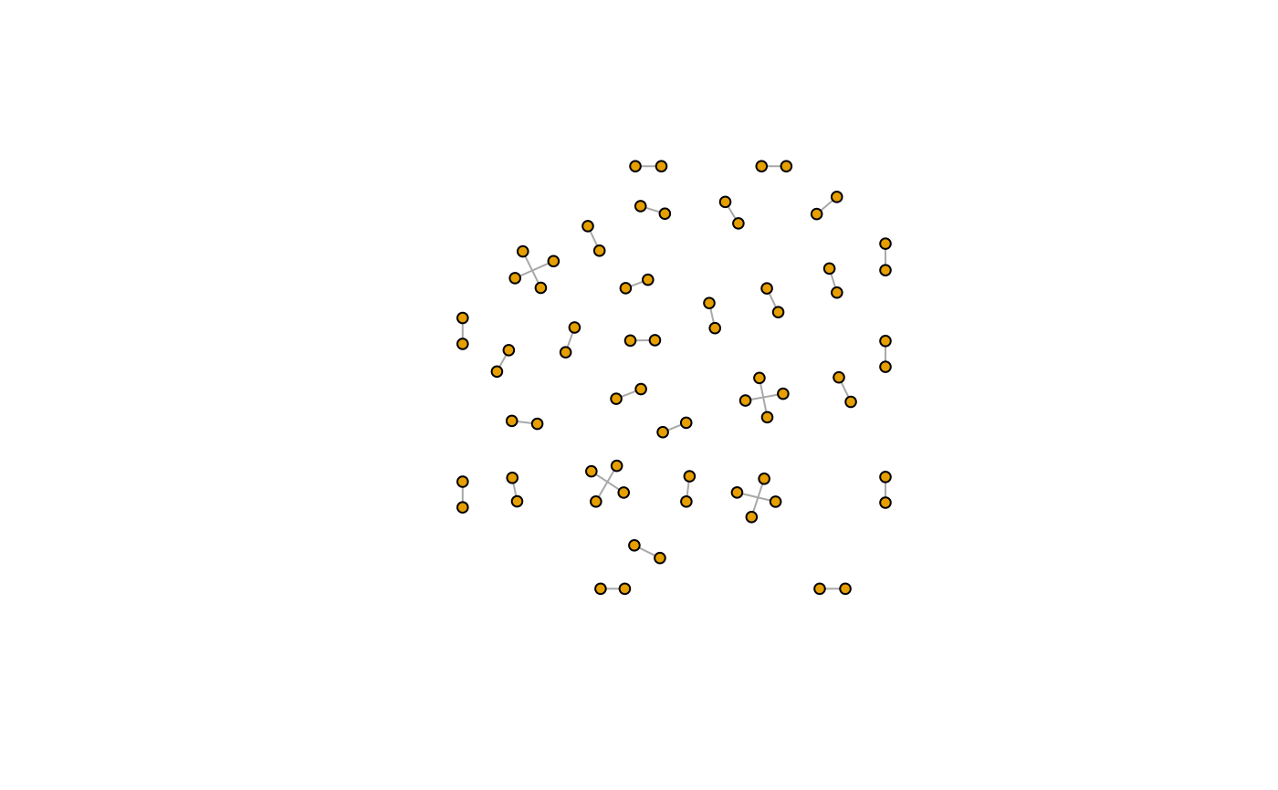
 g_4 <- make_empty_graph(n = 70, directed = FALSE) + edges(1:70)
plot(g_4, layout = layout_with_dh, vertex.size = 5, vertex.label = NA)
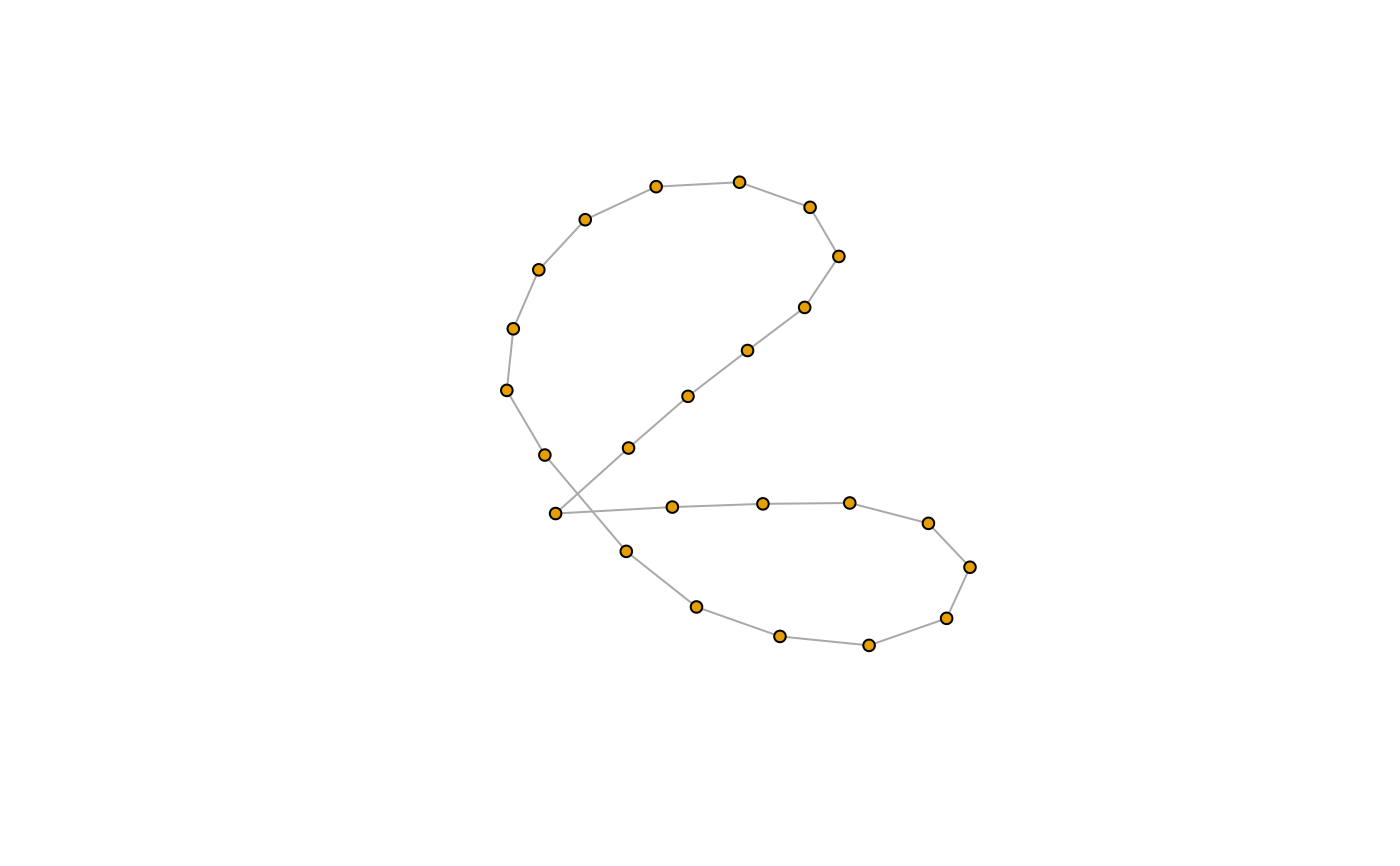
 g_5a <- make_ring(24)
plot(g_5a, layout = layout_with_dh, vertex.size = 5, vertex.label = NA)
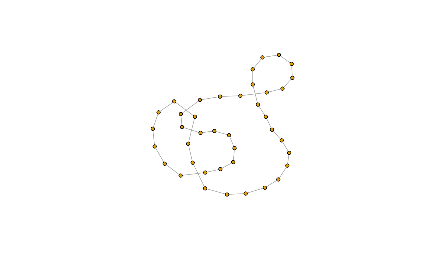
 g_5b <- make_ring(40)
plot(g_5b, layout = layout_with_dh, vertex.size = 5, vertex.label = NA)
 g_6 <- make_lattice(c(2, 2, 2))
plot(g_6, layout = layout_with_dh)
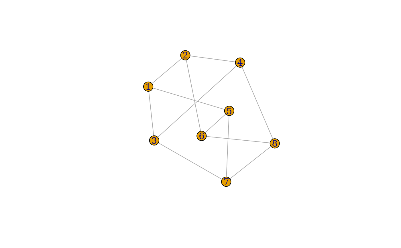 g_7 <- graph_from_literal(1:3:5 - -2:4:6)
plot(g_7, layout = layout_with_dh, vertex.label = V(g_7)$name)
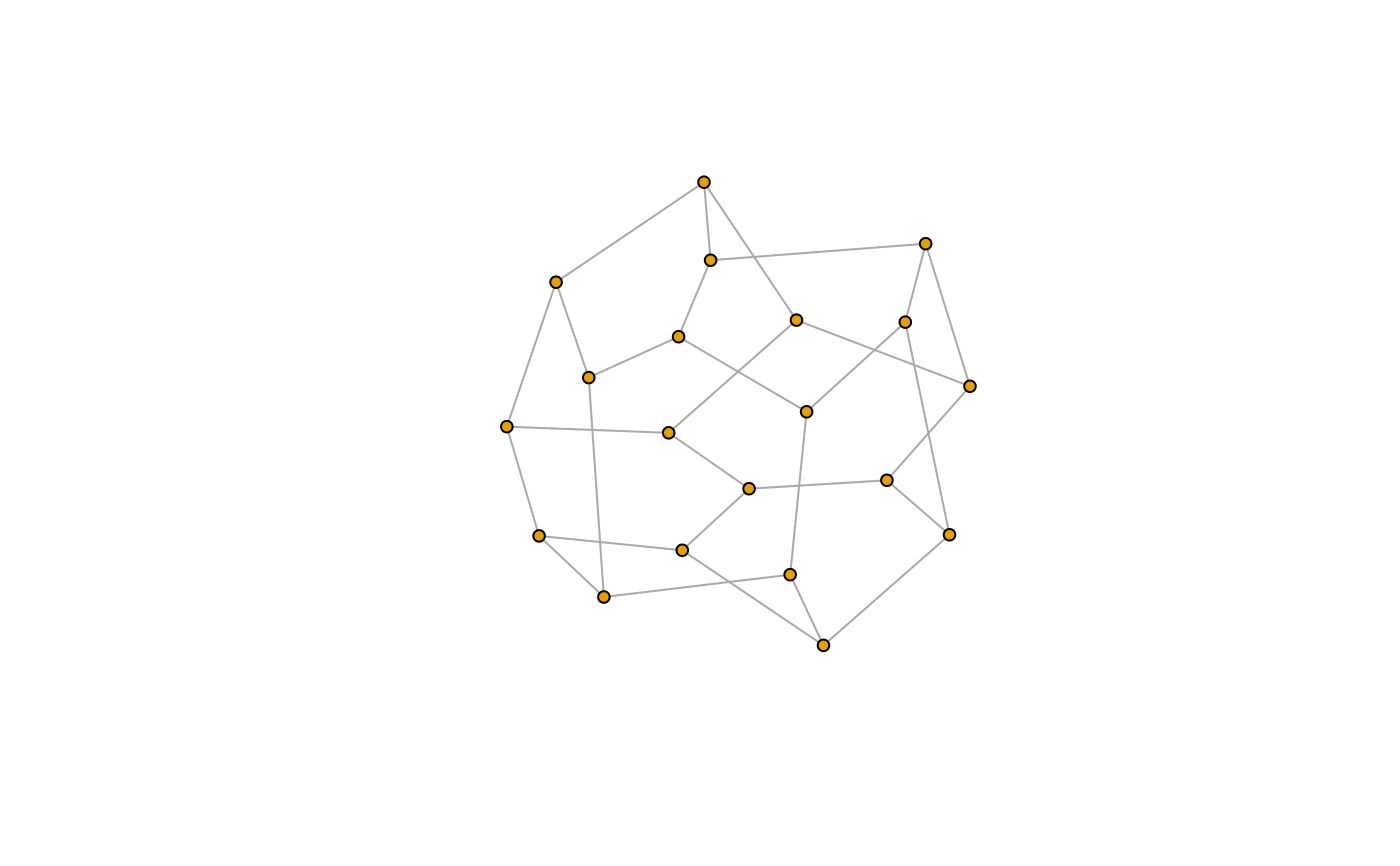
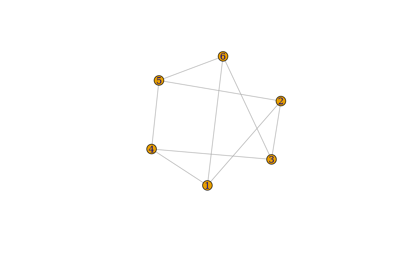 g_8 <- make_ring(5) + make_ring(10) + make_ring(5) +
edges(
1, 6, 2, 8, 3, 10, 4, 12, 5, 14,
7, 16, 9, 17, 11, 18, 13, 19, 15, 20
)
plot(g_8, layout = layout_with_dh, vertex.size = 5, vertex.label = NA)
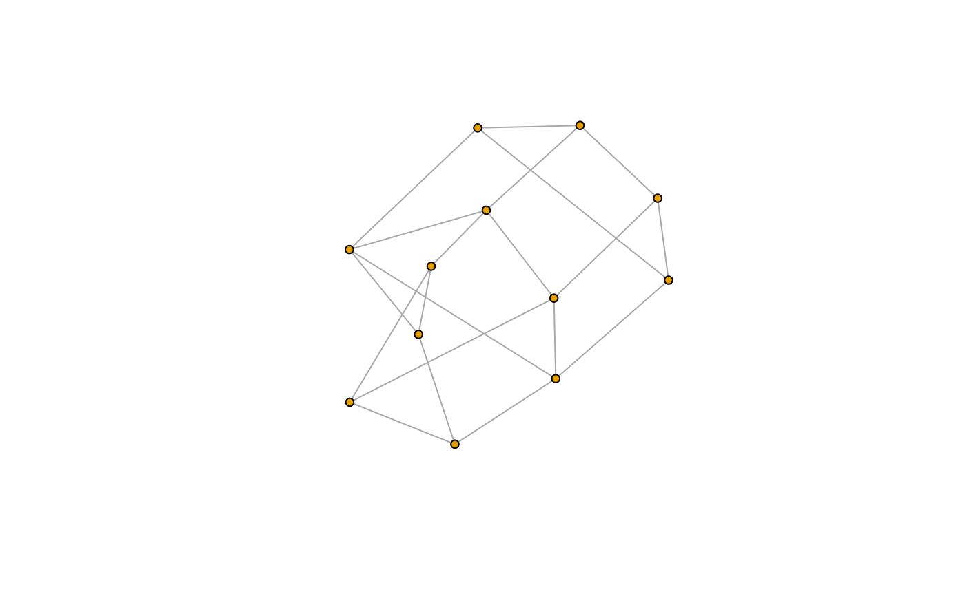
 g_9 <- make_lattice(c(3, 2, 2))
plot(g_9, layout = layout_with_dh, vertex.size = 5, vertex.label = NA)
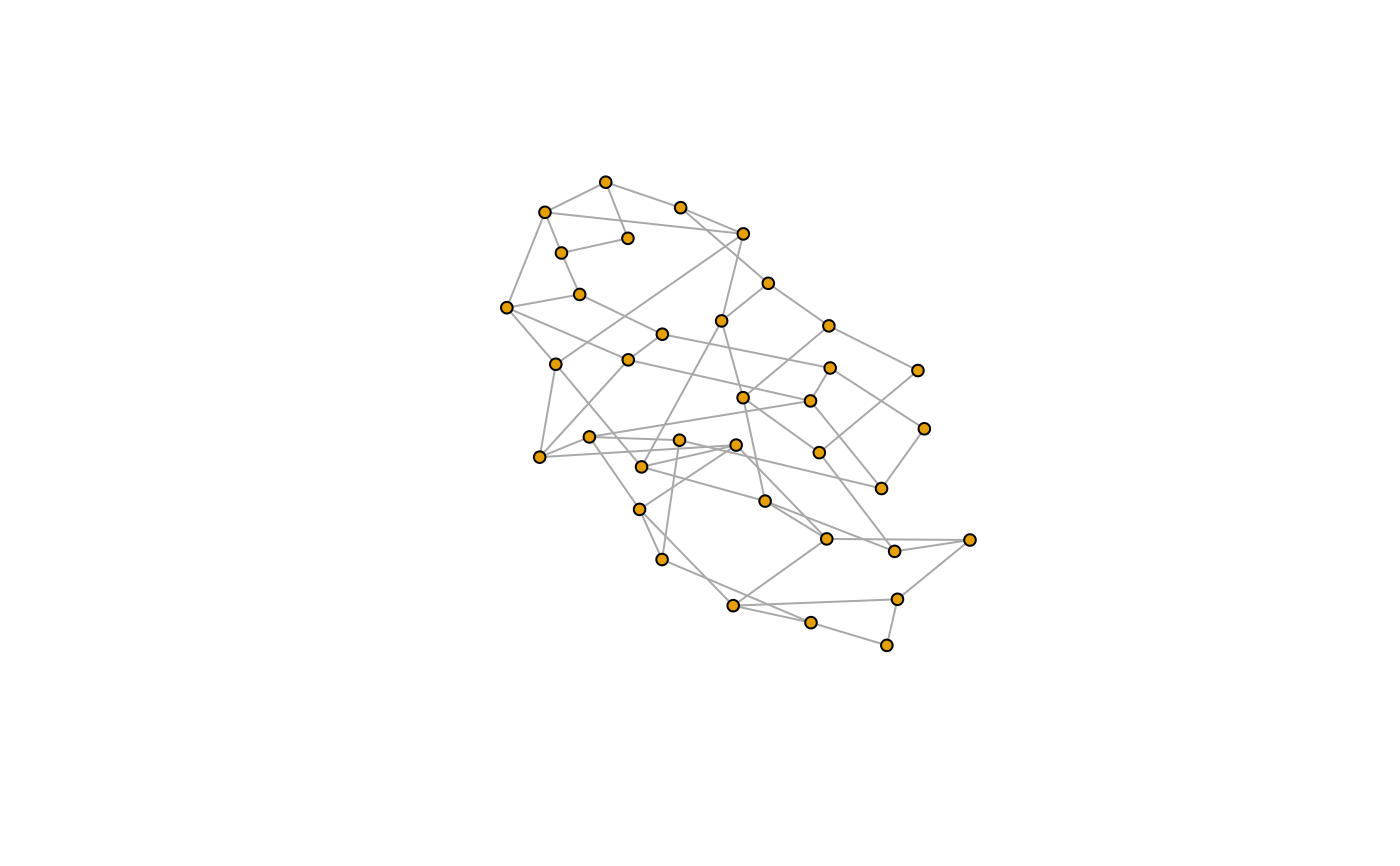
 g_10 <- make_lattice(c(6, 6))
plot(g_10, layout = layout_with_dh, vertex.size = 5, vertex.label = NA)
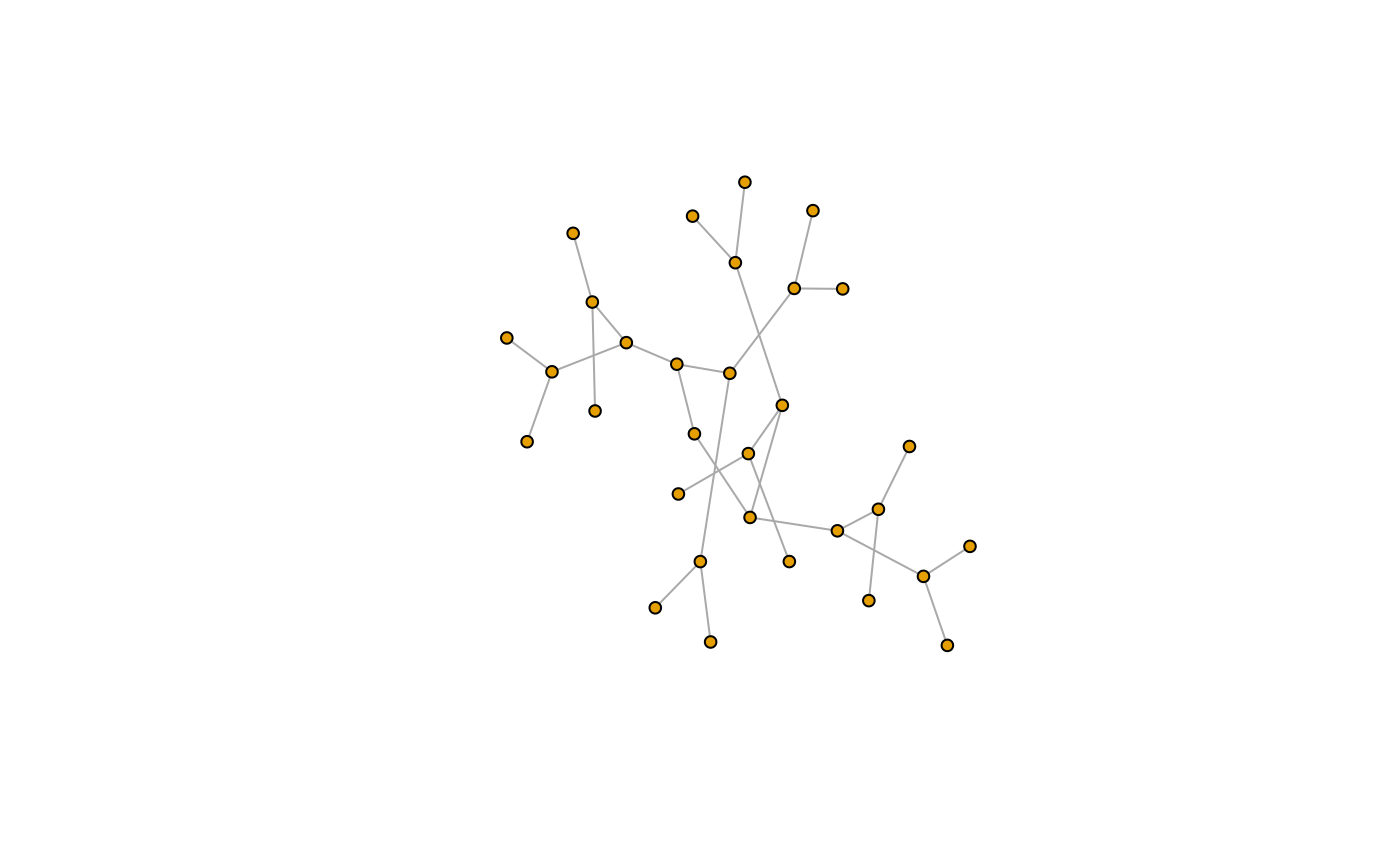
 g_11a <- make_tree(31, 2, mode = "undirected")
plot(g_11a, layout = layout_with_dh, vertex.size = 5, vertex.label = NA)
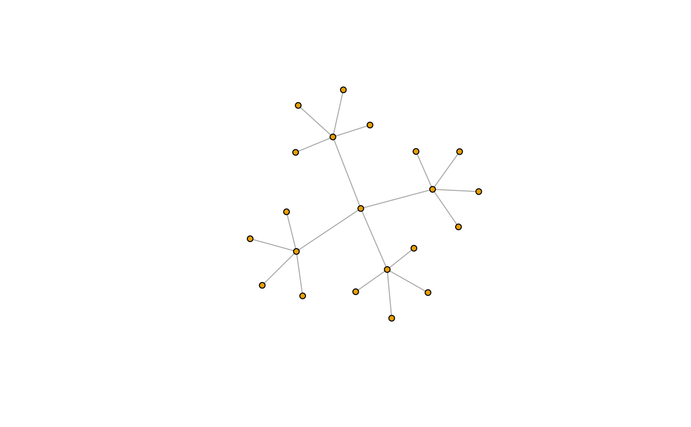
 g_11b <- make_tree(21, 4, mode = "undirected")
plot(g_11b, layout = layout_with_dh, vertex.size = 5, vertex.label = NA)
 g_12 <- make_empty_graph(n = 37, directed = FALSE) +
path(1:5, 10, 22, 31, 37:33, 27, 16, 6, 1) + path(6, 7, 11, 9, 10) + path(16:22) +
path(27:31) + path(2, 7, 18, 28, 34) + path(3, 8, 11, 19, 29, 32, 35) +
path(4, 9, 20, 30, 36) + path(1, 7, 12, 14, 19, 24, 26, 30, 37) +
path(5, 9, 13, 15, 19, 23, 25, 28, 33) + path(3, 12, 16, 25, 35, 26, 22, 13, 3)
plot(g_12, layout = layout_with_dh, vertex.size = 5, vertex.label = NA)
